 Hermit's Free Library MS-Excel
 Hermit's Free Library MS-Excel
Brief, but detailed introduction to spreadsheets and MS-Excel which covers using formulas including conditional statements and other functions, formatting, and graphs and charts. Explains features of the MS-Excel user interface and includes many tips on using MS-Excel effectively.
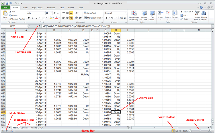
Important components of the MS-Excel program window include:
| Active cell |
Identified by dark border Displays results of any expression contained in the cell |
| Formula bar | Displays contents of active cell |
| Name box | Displays the cell reference for the active cell |
| Worksheet tabs | Select, add, delete, rename, reorder worksheets |
| Status bar |
Mode status: Ready or Enter (edit mode)
View toolbar Zoom control Caps lock, Num lock Right-click status bar to customize |
Spreadsheet files are called workbooks. MS-Excel 2012 and beyond workbooks (files) have the .xlsx file extension.
Much in the same way that the default name for a new Word document is Document1, the default name for a new Excel workbook is Book1.
By default, new Excel workbooks contain three worksheets, which are by default named Sheet1, Sheet2, and Sheet3. Worksheets are work areas where data and formulas are entered and results of calculations are displayed. Worksheets are represented by tabs at the bottom, left-hand corner of the Excel window.
New worksheets can be added, up to a maximum of 255, and worksheets can be deleted, renamed, and their tabs dragged and dropped into a desired order.
Worksheets are separate from each other, but formulas on one worksheet can access data which is on another worksheet. For example, if we have four worksheets, each representing quarterly earnings, those earnings could be added together and displayed on a fifth, summary worksheet. As we'll see below, when one worksheet references a different worksheet, it's called a three-dimensional reference.
The worksheet work area is divided into rows and columns, like a grid, or table. Rows and columns have headings to identify uniquely each row and heading. Numbers are used as row headings, and letters are used as column headings. Column Z is followed by columns AA, AB, AC, etc..
New rows or columns can be inserted anywhere they are needed, and they can also be deleted, but the overall grid is always 65,536 rows by 256 columns.
The intersection of a column and row is a cell.
Cells are referenced by the combination of their column letter and row number. The first cell on a worksheet, located in the upper, left-hand corner of the worksheet area, is referenced as cell A1. Cell references are used to tell formulas which numbers to use in their calculations.
Spreadsheets wouldn't be very useful if we had to manually correct cell references each time rows or columns were added or deleted, or copied or moved. Instead, spreadsheets are programmed to have a special awareness of cell references, and automatically adjust references to accommodate nearly any kind of change we can make to a worksheet.
There are actually four different variations of cell references. The default reference is the relative reference. Relative references make it possible to enter a formula in one cell and then reuse the formula in other cells without having to re-write it to fix up the cell references.
When a formula containing relative references is copied, Excel automatically adjusts the references in the destination cell by incrementing or de-incrementing them once for each displaced row and/or column.
Consider the illustration below, in which the relative cell references A1 and B1 are copied from the source cell C1 to cells D1, C2, and D2.

At the other end of the scale are absolute references. Excel will not tinker with absolute references when they are copied or moved: they always point to the same cell. An example of an absolute address is $A$1.
The other two types of cell references are called mixed references. Mixed references are half relative and half absolute. Examples of mixed references are $A1 and A$1. When the $A1 reference is copied, Excel can adjust the row (1), but not the column ($A). Conversely, for A$1 the column can be adjusted, but not the row. So the $ tells Excel "leave this part of the reference alone, don't adjust it under any circumstance".
When entering absolute or mixed cell references you can type in the dollar signs where needed, or you can use the F4 key. In edit mode, the F4 key cycles through each reference variation at the cursor position. With the cursor in the reference A1, four successive taps on F4 will produce $A$1, A$1, $A1, and then back to A1.
Cell ranges are groups of cells. Cell ranges can be cells arranged in rows, columns, or blocks, as long as they are all together.
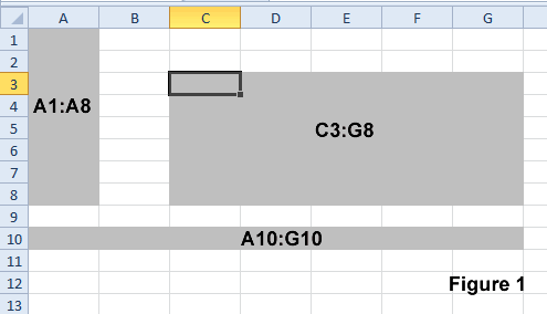
A cell range is referenced by the cell reference for its first cell and the cell reference for its last cell, separated by a colon. For example, the cell range reference for the first 8 cells of column A is A1:A8 (Figure 1). The reference for the cell range consisting of the first 7 cells in row 10 would be A10:G1.
Ranges for continuous blocks of cells are defined by the references for their upper left-hand and lower right-hand (or lower left-hand and upper right-hand) corners. See C3:G8 in Figure 1.
A cell range specifies the data for use by formulas and functions. For example, to add up the contents of cells A1, A2, A3, A4, and A5 using the SUM() function (more in a moment), the formula is =SUM(A1:A5).
As in selecting text in Word, we frequently select ranges of cells in Excel in order to format them or copy or move them.
The following table summarizes the types of contents cells can
have. More detailed explanations follow.
| Text |
Text data Labels (descriptions of data) |
Text data includes digits: Phone numbers Zip codes Credit cards |
Signaled by ' |
|
|
|||
| Formulas |
Numbers Cell references Math operators Functions |
Cell references: Absolute, mixed, or relative 3-dimensional |
Signaled by = |
|
|
|||
| Values | Variables or constants |
Formatting No decimals (3) Decimals (3.14) Currency ($3.14) Percentage (3.14%) Scientific (1.275E2) |
|
|
|
|||
| Dates |
Short date: 01/01/2009 Long date: January 1, 2009 |
Dates are stored as numbers 1 Jan 1900 represented by 1 |
|
|
|
|||
| ####### |
Displayed when column is too narrow to accommodate data |
Widen column to display data | |
If you select a cell and just begin typing, Excel makes some assumptions about what you are entering. If you begin with an alphabetic character, Excel assumes you are entering text and treats the contents as such. If you begin by typing a digit, Excel assumes you are entering numbers.
Works well often, but not always.
For example, if we try to enter a formula that subtracts the contents of one cell from another by just typing A1-A2 into a cell, Excel enters it as text, not a formula. Instead, we signal to Excel that we want a formula and not text by beginning with an equal sign: =A1-A2.
And digits that we want Excel to store as text and not numbers are another problem.
Take phone numbers and zip codes, for example. They should be entered as text, not numbers. After all, we're never going to do math with them. Also, as numbers Excel would right-align them instead of left- aligning them as text.
Another important example of this would be credit card numbers. Most credit card numbers are sixteen-digits long. Since Excel stores numbers to only 15-digit precision, a 16th digit would be changed to a zero.
In all such cases we signal to Excel to store the digits as text and not numbers by beginning our entry with an apostrophe.
A spreadsheet formula is a mathematical equation used to calculate a value. Formulas can include values, references to other cells, functions, and math symbols. As mentioned above, you must always begin entering a formula by typing the = sign. If not and the formula begins with an alphabetic character, Excel treats it as text and makes no calculation.
Values are just what you'd expect, i.e. numbers.
Note that Excel is a bit tricky about displaying numbers. Sometimes it seems to be short-changing numerical values by rounding them off. Fear not, this is just a sleight of hand on the part of Excel to make it easier for users to digest decimal numbers.
Consider the following example:
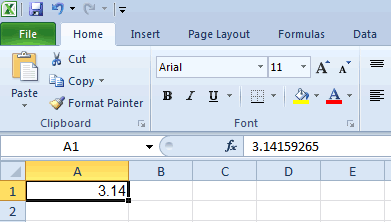
| We enter 3.14159265 in A1, but that cell's been formatted to show only two decimals. |
|
| Are the decimals gone? No. Look up at the Formula Bar and you see that A1 actually contains 3.14159265. | |
| When making calculations, Excel always uses all available decimals (up to 15-digit precision) |
Variable values are frequently used in spreadsheets. Examples of variables are the price of gas, the rate of inflation, a currency exchange rate, or, as in the example below, sales tax percentages.
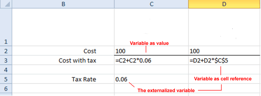
By definition, a variable value is subject to change. If we use variable values directly within cells, as the .06 in cell C3 of the illustration below, we create a potential problem.
If, as is often the case, we use a variable in more than one cell, when its value changes, we need to remember all and update them individually. Not the way to go.
Instead, externalize the variable. Instead of putting its fleeting value in formulas or expressions, put the variable value in its own cell and use its cell reference wherever its value is required.
Externalized variables are easy to update from one, clearly identified and easily found location.
To see an example of an externalized variable, look at cells C3 and D3 of the worksheet snippit below.
Notice the dollar signs in the reference to cell C5. They
make the cell reference an absolute reference instead of a
relative one. Absolute references are 'hard-wired'. If we copy or
move a formula with an absolute reference to another cell, that
reference is never adjusted for the new location - it always
absolutely points to the original cell.
|
Externalized variables play many important roles. One of the most useful is in supporting a What-if Analysis.
A What-if Analysis is used to assess what effect changing one or more variables has upon the outcome of a calculation. For example, What-if a loan's interest rate is lowered by two percent? Or, What-if the down payment is increased by one thousand dollars? What would be the effect of those two scenarios upon the loan's repayment?
Spreadsheets represent dates using serial numbers. For example, Excel represents January 1, 1900 (the oldest date Excel can represent without outside help) with the number 1. January 2, 1900 is represented by the number 2, and so on and so forth.
Although it sounds odd, this method of representing dates makes it possible for a formula to compare two dates to see which one came first, or to subtract one date from another to determine the number of elapsed days. Likewise, days can be added to a date in order to determine the date so many days in the future. This is very useful in accounting and many other applications as well .
All spreadsheet programs include functions. Functions are pre-set, named formulas designed to obtain a specific result based on the data provided to them. There are functions to solve financial, scientific, and trigonometry problems, as well as functions that work with text, dates and time, and logic.
All functions follow the same format, which is the name of the function followed by a set of parenthesis. The parenthesis enclose the function's argument(s). Arguments are the numbers, text, or cell references a function uses to perform an operation and return some value. Many functions take a single argument (frequently a cell range) but others can require several arguments.
The most commonly-used functions are the
math functions. Math functions calculate things like sums,
averages, and largest or smallest number in a list of values.
| Math Function | Returns | |
| SUM() | Sum of numbers in a range | |
| AVERAGE() | Average of numbers in a range | |
| MODE() | Value which occurs most frequently in a range | |
| MIN() | The minimum value in a range of numbers | |
| MAX() | The maximum value in a range of numbers |
The sum() function is probably the most widely-used function of all. Sum() adds up the numbers contained in a range of cells. If we want the sum of all the numbers in the cells from A1 to A10 to appear in cell A11, we select cell A11 and type in:
=Sum(A1:A10)
The = tells Excel that what's coming is a formula, Sum tells it the name of the formula, and (A1:A10) tells it what numbers to add up. When we press Enter, Excel enters the formula, performs the calculation, and displays the result in A11.
If we wanted to know the average of all the numbers in the range A1:A10, we'd use the average function:
=Average(A1:A10)
The greatest number in the A1:A10 range:
=Max(A1:A10)
Functions can also be a part of a longer formula:
=Sum(A1:A10)*B1/Average(C1:C15)
Today(), the most commonly used date function, is an example of a function which has no arguments. Enter "=today()" into a cell and the cell displays the number representing the current date formatted as a date. If you want the cell to display the current date and the current time, enter "=now()".
Functions are key to using spreadsheets effectively. Begin by learning how to use the basic math functions and then expand your repertoire as your spreadsheets become more sophisticated.
Excel Help does an excellent job of explaining all the functions. You can browse the functions by category and see what each one does. To learn more about a specific function, read Excel's description of the function's purpose and its arguments, and examine the examples given. And you can copy and paste examples right into a live worksheet for experimentation.
Once you've entered a formula containing a function, Excel will automatically adjust the function's arguments to accommodate changes you make to the worksheet. Take the example of Sum(A1:A10): if we were later to insert five rows anywhere between A1 and A10, the formula would change from =Sum(A1:A10) to Sum(A1:A15).
A final note worth mentioning: when you enter the name of a function correctly in a formula in lower case, Excel changes the function name to upper case when you press Enter. If the name doesn't change to upper-case, what you typed is not the correct name for a function.
Summary of math, comparison, and logical operators used in spreadsheets:
| Math |
+ Addition - Subtraction * Multiplication / Division ^ Exponentiation |
|
|
|
| Comparison |
< Less than <=Less than or equal to >Greater than >=Greater than or equal to = Equal to <>Not equal to |
|
|
|
| Logical |
#NOT# Logical Negation #OR# Logical Or #AND# Logical And |
Many people have been introduced to the Please Excuse My Dear Aunt Sally method of remembering the standard order of precedence: Parenthesis, Exponents and roots, Multiplication and Division, and Addition and Subtraction.
The Aunt Sally method is fine as long as you don't fall into the trap of believing that Multiplication comes before Division and Addition comes before Subtraction. They don't, at least not necessarily.
All expressions enclosed within parenthesis are evaluated first. Within, or in the absence of parenthesis, multiplication and division are carried out from left to right before addition and subtraction. Next, addition and subtraction are carried out, from left to right.
For example, look at this expression:
44 / 2 * 3 - 2 + 10
The correct evaluation of this expression is to first divide 44 by 2 and then multiply that by 3. The multiplication operation is not performed before the division because from left to right the division comes first.
Because, left to right, the subtraction comes before the addition, it is performed next. Finally, the addition operation is performed.
Conditional statements are expressions that use one or more comparison operators. Example of a conditional statement:
2
Conditional statements evaluate to either True or False. The conditional statement 1>2 obviously evaluates to False. Conversely, the conditional statement 2>1 is True.
The most common use of conditional statements on worksheets
is with the IF() function. The IF() function evaluates a
conditional statement in order to decide between two possible
courses of action. For example: if a payment is overdue, add a
late fee, otherwise do not. Here's how it works:
Normal View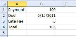
|
Formula View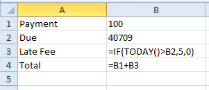
|
The figure above shows two views of the same portion of a worksheet.
First, note that the date 6/15/2011 in B2 on the left appears as the number 40709 in cell B2 on the right. As previously mentioned, dates are represented by numbers in spreadsheet programs. Forty-thousand, seven-hundred and nine days elapsed between January 1, 1900 and June 15, 2011.
Next, in the Formula View, see that cell B3 contains a formula and not a number as it appears in the Normal View.
=IF(TODAY()>B2,5,0)
The IF() function returns one of two possible values (5 or 0) depending upon whether or not the condition TODAY()>B2 is true. If the condition is true, the value in B3 becomes 5. If the condition is false, the value in B3 becomes 0.
TODAY(), which has no arguments, is the date function that returns the current date, without the time. The IF() function uses the GREATER THAN comparison operator (>) to see whether the due date (B2) comes before or after the current date as reported by TODAY(). If the due date is after the current date, then the condition is TRUE and the value in B3 becomes 5.
If the date in B3 was not greater than the date in B2, the IF() function's conditional statement would evaluate to FALSE, and cell B3 would become 0.
Finally, the formula in cell B4 adds the payment amount (B1) to the late fee (B3), which is either 0 (zero) or 5 (five) according to the IF() function.
The ability of the IF() function to decide between two courses of action based upon a condition is called branching logic. Branching logic is the cornerstone of many spreadsheets.
To enter a formula or data in a cell, or to edit the cell's contents, you must first select it to make it the active cell. Often the easiest way to do this is to click in the cell using the mouse, or use the keyboard's arrows, PgUp, PgDn, Crtl-Home, Ctrl-End, etc..
Those techniques work well when you are already near the cell you want to work with, but when the cell is at a distance there are two other techniques which save the effort of getting your bearings and navigating to the new location.
Voila! Either way, you're there!
It's important to fully understand the interesting and productive variations available in spreadsheets for selection and copy and paste.
First of all, we need to correctly differentiate between
Excel's Regular mouse pointer, Fill Handle mouse pointer,
and the Fill Handle.

|

|

|
|
Regular Mouse Pointer |
Fill Handle Mouse Pointer |
The Fill Handle |
The regular mouse pointer is used to select a range of cells by left-dragging through them. To select two or more independent, non-adjacent cell ranges at the same time, select the first range and then hold down Ctrl while you select the other(s).
Once a cell range has been selected, its contents can be copied to the Clipboard (Ctrl-C) and then pasted (Ctrl-V) from there to the desired destination. Note that the selected destination need not match the source selection, it is sufficient to select only the cell in the upper, left-hand corner of the destination cell range.
The Fill Handle mouse pointer appears when you hover over a cell's Fill Handle. The Fill Handle is a small black square in the lower, right-hand corner of the selected cell (see figure above).
Depending upon circumstances, the Fill Handle can perform two different types of operations in a spreadsheet: Copy or Fill.
Copy
If you want to copy the contents in the range of cells A1:A5 from column A to column B, use the Fill Handle this way:
Fill
When Excel recognizes the contents of the source cell or range of cells
as a single value or series of values which are ordinal, it continues
filling the series in the destination.
| Ordinal Values | Ordinal series |
| Mon | Mon-Tues-Wed-Thu-Fri-Sat-Sun |
| Jan | Jan-Feb-Mar-Apr-Jun-Jul-Aug-Sep-Oct-Nov-Dec |
| 9:00 | 9:00-10:00-11:00-12:00-1:00-2:00 |
| 1st Grade | 1st Grade 2nd Grade 3rd Grade 4th Grade 5th Grade |
So, if you enter "Mon" in a cell and then drag that
cell's Fill Handle across the next six cells in either the column
or the row, Excel will fill them with "Tue-Wed-Thu-Fri-Sat-Sun".
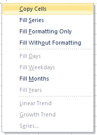
| But what if you actually want to copy a cell's contents and Excel thinks it's an ordinal value and wants to fill the series? In such a case you can modify the Fill Handle's default behavior by right-dragging instead of left-dragging. Right-dragging and then releasing the mouse button summons a shortcut menu. |
|
| Now you can choose exactly which action you want Excel to take. | |
| Note the Fill Without Formatting choice. This option copies the contents of cells, but retains the formatting of the destination cells. |
AutoComplete is very useful under some circumstances, but often it's just a distracting PITA. It can be turned off in Excel Options >Advanced (/TOA).
Accountants are usually busy people. They're not into wasting time. Below is a short list of keyboard shortcuts that most accountants would regularly use. All of them are for tasks every user needs in spreadsheets.
Keyboard shortcuts are a fast and efficient alternative
to using the mouse. Perennial favorites include Home,
Ctrl-Home, Ctrl-A, and Ctrl-C-X-V. Here's a few more.
For an even more comprehensive list of keyboard shortcuts in Excel,
look here.
| Keystroke | Action |
|
|
|
| F2 | Enter Edit mode |
|
|
|
| F5 | Goto |
|
|
|
| Alt= | Autosum range |
|
|
|
| Ctrl` | Formula view |
|
|
|
| Ctrl-F | Find |
|
|
|
| Ctrl-Shift-8 | Select cells in proximity to selected cell |
|
|
|
| /oe | Format cells dialog |
The final keyboard shortcut in the previous list, /oe, belongs to an entire set of spreadsheet keyboard shortcuts developed for the venerable Lotus 1-2-3 spreadsheet and known as the Slash commands.
In those days before mice were invented, Slash commands were the centerpiece of the ground-breaking Lotus 1-2-3 user interface. Users navigated the Lotus menus and accessed program commands by pressing the slash key (/) and then typing one to four letters which were linked mnemonically to the their commands. The approach was stunning for its simplicity and its speed and effectiveness.
Lotus 1-2-3 is long gone, but its Slash key interface remains to be an undocumented feature of every spreadsheet program up to this very day.
One example of a slash command is /oe. Opens the Format Cells menu. While the mnemonics sometimes seem to be a little wonky, they are easy to remember and use.
You can append number, alignment, font, or border to /oe to access those deeper menus and commands.
Note that the slash (/) key is "sticky". Just tap it and Excel leaps to attention, waiting for you to type letters corresponding to the a command. To cancel the operation after you've begun, you simply tap the Esc key.
A good example of a useful slash command is /toa. This command Opens Excel Options to the Advanced screen. The O and A, of course, are for Options and Advanced, but are you puzzled by the T? In Lotus 1-2-3, T stood for the Tools menu. MS-Excel's Ribbon interface has no Tools menu, but it lives on as a phantom stop along the original 1-2-3 slash command interface.
If you enable the slash commands (Options >Advanced >Lotus Compatibility) in MS-Excel 2010 you'll be able to use the slash key in place of Alt to access Excel's 'keyboard accelerators', which make virtually every Excel command accessible from the keyboard.
Normal view is the mode most commonly used to create, edit, and format worksheets, as well as to view worksheet results.
Formula view is essential for auditing worksheets and tracking down formula errors. Unlike Normal View, which displays the results of formula calculations, Formula view displays the actual formulas contained in worksheet cells.
Switch to Formula view by holding down Ctrl and pressing the accent key. The accent character looks like an apostrophe that is about to fall over backwards (`) and on standard PC keyboards it's up in the left-hand corner on the same key with the tilde (~).
When you want to look at two places on a worksheet at the same time, go to the View tab, Window group, and Split the Window.
For large worksheets you can use Freeze Panes to keep row or column headings in view while you scroll through the data. Freeze Panes is in the Window group of the View tab. You can freeze just the first row or first column, or you can freeze both rows and columns. When freezing rows and columns, begin by selecting the cell in the upper, left-hand corner of the area you want to scroll - rows above and columns to the left will be frozen.
Right-click worksheet tabs to color-code them. Can be developed in a systematic way: yellow for documentation, blue for summary worksheets, etc..
After setting up a complex view, including freeze panes, split window, or hidden rows or columns, give it a name and save it as a custom view.
Once saved you can switch to a Custom view instantly, without having to do and undo all the set-up steps.
Warning. Always create a Normal view before you begin so that you can return to the basic view.
An example of a custom view would be to audit a worksheet: open the worksheet in two windows, worksheet results in one window and a zoomed formula view in the other. Once the two window views are set up, save the whole thing as a Custom view (or a workspace if more than one workbook is involved - see below).
Custom views are opened, closed, added, and deleted using the Custom View menu in the Workbook Views group of the View ribbon tab. You can access the Custom View menu by typing /VV (victor victor).
By default, Excel opens multiple workbooks in separate document windows of the same program window. This setting makes it impossible to view two spreadsheets on the screen at the same time.
However, configuring workbooks to each open in their own program window allows them to be tiled and viewed simultaneously.
To make workbooks open in their own program windows:
After setting workbooks up to open in their own program windows (previous section), you can tile them this way:
Hide rows or columns when they contain data which is required for calculations, but distracting to display.
Use these steps to hide rows or columns:
Password protection is optional, if you use it don't forget the password!.
Pressing Enter to complete data entry or an edit usually causes the cell selector to move to an adjacent cell. You can control what direction Enter makes the cell selector move or even make the cell selector remain in the same cell.
Whatever direction you make the cell selector move when you press Enter, Shift-Enter will move it in the opposite direction to that .
The Arrow Keys can also be used to complete data entry and move the cell selector in the direction you want.
To choose which direction the cell selector moves for the Enter key:
You can get to Advanced options much faster by typing the /toa slash command.
What direction its best to have the cell selector move depends upon the nature of the worksheet layout and what you are doing at the moment.
Using /toa makes it so quick and easy to adjust the movement to match your work rhythm that it's worth doing on an ad hoc basis.
A final thought on data entry and cell selector movement. The Tab and Shift-Tab keys always move the cell selector left and right. Therefore, if you make down the default direction for Enter, you can use Enter to move the cell selector down, Shift-Enter to move it up, Tab to move it right, and Shift-Tab to move it left.
To enter or modify data rows in a spreadsheet in a form view:
In form view you can also move from record-to-record to edit or search for a record based on criteria.
When using the keyboard to fill in data for a range of cells, selecting the range first will conveniently restrict the cell selector to that range.
To break out of the range, press any arrow key on the keyboard, or select another cell or range of cells with the mouse.
To fill an entire range with the same value:
The nature of spreadsheets is that they are easily altered, either intentionaly or inadvertently. Inadvertent changes to data and formulas can damage a worksheet's integrity and potentially do great harm. Fortunately there is a way to protect worksheet cells from unintended changes. It's a two-step process: Lock and Protect.
The first step is pretty much automatic because by default all worksheet cells are Locked. You'd think that would be it, but locked cells aren't protected until a user carries out the second step, which is to apply Protection to them.
The second step is accomplished by selecting the Protection option in /TPP (Tools, Protection, Protect worksheet) or /TPW (Tools, Protection, protect Workbook). Once Protection is applied, no changes can be made to worksheet cells which are both locked and protected.
Why is cell protection designed this way? The short answer is to provide flexibility. The duo of Lock and Protect give the least cumbersome way to protect that which needs it, while still allowing changes to the data-entry cells.
Imagine a workbook with several large worksheets, all but one of which contain only unchanging or rarely changing data. The remaining worksheet has many formulas and a few data-entry cells scattered around it.
Since all workbook cells have been Locked by default, we only need to unlock the data entry cells (/OEP) and then apply Protection to entire worksheets (/TPP), or the whole workbook (/TPW).
If it becomes necessary to make changes to other cells, all we need to do is temporarily remove Protection from a worksheet or the entire workbook.
Documentation is very important. Conventionally, the first worksheet is used to document the overall workbook. Minimum documentation should include:
In addition, document special features and information which would be useful in the future to either the author or other users. This might include a history of worksheet modifications.
While the purpose of each worksheet should be described in the documentation worksheet, it's still a good practice to give descriptive names to worksheets (right-click worksheet tab and select Rename) instead of the generic Sheet1, Sheet2, etc.
It's also good spreadsheet etiquite to include a descriptive title in the first row of all worksheets. The worksheet title can be made more attractive using font size and color, and centering them over multiple columns using the Merge and Center tool.
The layout of a worksheet is how data is organized into its columns and rows, which can also be referred to as fields and records.
A field is where one of an entity's attributes is stored. Examples of fields are description, stock number, price, color, size, and quantity.
The collection of all the fields (attributes) for one specific entity (a stock item for example) is referred to as a record.
Since worksheets have way more rows than columns, and there are usually more records (items) than fields (attributes), it is customary to use columns for fields and rows for records.
If there should be more fields than records in a set of data then it makes sense to reverse the standard configuration.
For example, in the case of a comparison between loans from two different lenders, there would be more fields than records. Then it would make sense to put the fields (loan amount, money down, interest rate, number of payments, amount of each payment, etc.) in rows and the records (Lender #1 and Lender #2) in the columns.
In general, use worksheet layouts and page orientations that use space efficiently and make the data easy to interpret.
Most workbooks represent data in two dimensions, but data can also be recorded and viewed three-dimensionaly.
For example, a 2-D model would accomodate tracking a company's annual sales, expenses, and profitability. We would place the financial data in rows and use columns for each month of the year.
But suppose we want to represent and analyze several years' worth of data. Picture those separate 2-D worksheets for each year stacked on top of each other and you get a third dimension: depth.
Using the same workbook for all the years makes it convenient to analyze them in their aggregate. We can write formulas on a separate worksheet that draws data from individual annual worksheets for a summary.
For this we use 3-D cell references. 3-D references include designations for row, column, and worksheet. Look at this 3-D reference for the first cell on a worksheet named Finances_2010:
Finances_2010!A:1
The exclamation point delimits the worksheet name from the cell, just as a colon (:) separates the column from the row in the cell reference.
Warning! If you name a worksheet with an embedded space like this:
Sales 2010
and then try to reference one of its cells like this:
Sales 2010!A:1
Excel hits the wall when it encounters the embedded space. You'll have to use this format:
"Sales 2010"!A:1
or eliminate the embedded space problem with names like Sales_2010.
Too many currency symbols on a worksheet creates distracting clutter. According to standard accounting practices, currency symbols should only be used on the first and last rows in a column of currency numbers. Used this way they identify the nature of the number column (top row), and draw attention to the "bottom line" (last row).
(If data is oriented in the other sense, use the currency format for the first and last columns instead).
One oddity of Excel is that currency symbols can be added to numbers using the Accounting format button on the Ribbon, but the same button will not remove them. To do that you must open the formatting dialog box.
When decimal points of numbers in columns don't line up it's probably because their cells have different number formats: currency versus accounting, for example. Here's why:
Negative numbers can be displayed either in red, or in parentheses (), depending upon the number style used. When parenthesis are used, Excel reserves a space for the trailing ")". Numbers formatted that way are shifted one space to the left from numbers formatted with red for negative. The result: mis-alignment of the decimal points. The solution is to use the same number format style for all numbers in the same column.
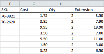
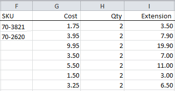
By default, spreadsheet programs left-align text, a
conventional arrangement that works well for row labels, but
which can create problems for columns labels. Because numbers
are right-aligned by default (in order to line up their digits
properly), left-aligned column labels can end up having poor
proximity with the data with which they are associated.
Example:
Text justified left (default)
|
Text justified right
|
The solution is to use right or centered text alignment to place labels in better proximity to the numbers.
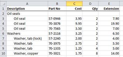
Indenting text can be used to create the effect of
subsections as in the example below.
As previously explained, spreadsheets keep track of dates as numbers. When you encounter the situation in which Excel displays a date after you have enter a number (or visa versa), it just means the cell has been formatted the wrong way. Just apply the appropriate format.
Because MS-Excel represents dates as numbers, their formats can be changed at any time. Contrast this with MS-Word, whose dates are just text and whose formats can only be changed by deleting and re-entering them. (Unless you know the clever technique of sending data on a round-trip from Word to Excel and back again. To see how, check out this exclusive Hermit Brain Teaser).
Sometimes, a visual representation of data is the most striking and effective way to convey the meaning of the numbers.
A chart is a combination of text and graphics that together present a visual portrayal of numerical data.
A graph is the actual visual representation of the data, while other parts of the chart include labels for the axis, tick marks (divisions on the axis), and a legend to identify the data sources. Data sources are the worksheet ranges containing the data represented by the graph.
Charts should not only be visually attractive and easy to interpret, they should be accurate. In addition to being based upon accurate data, the graphs themselves should portray the data in a manner that represents its true nature.
The space used by a chart's graph, title, and legend is referred to as the chart area. Inside the chart area is the plot area that holds the graph.
A chart can be embedded on a worksheet with its source data (the default in Excel), or as part of data summary worksheet, or it can be placed on a separate worksheet, alone or with other charts.
As visual aids during presentations, charts can be very effective. Charts can be added to Powerpoint slides in several ways.
OLE gives charts automatically update to reflect changing data in an Excel worksheet.
Following are some of the guidelines offered by Strategic Communications on their website. While intended for presentation charts, the same principles apply to resident workbook graphs and charts.
As with graphics, you must select a chart object before you can work with it. When you want to de-select a chart object, press the Esc key.
First, a little trick in Excel. If you select a range of data and its labels, and then press F11, Excel will insert a column chart on its own chart sheet. The resulting graph chart is austere, but serves up a quick way to take a reading on numbers visually. It would be nice to press Ctrl-Z and have the graph go away after a quick observation, but actually you will have to select the worksheet's tab (Chart 1) and press Del.
Line graphs show trends. They plot changes to one or more data categories over a period of time. Ideally, the time intervals should be identical. The convention is to plot time on the horizontal (x) axis, and the data on the vertical (y) axis.
Examples: Daily stock prices or maximum temperature readings for July; increase in cellphone usage between 2000 and 2012.
Column (vertical) and bar (horizontal) graphs use height or length to compare several different groups or categories of data. Columns are more conventional but bars are sometimes more analogous than columns; example of time (duration) which culturally we interpret from left to right.
Examples: Charitable donations collected by High School A, High School B, and High School C; the time it took for three brands of antacid to dissolve in water.
Pie charts show proportion, they use area to compare parts of a whole. Pie and time do not mix well. When sliced too thinly, pie becomes messy and less effective. Exploded pie is particularly messy, depending on the filling, but useful to emphasize or highlight one or a few slices out of the whole. Pies can only represent 100 percent of anything, no more, no less. When pie is tipped and/or rotated, resulting perspective becomes an impediment to correct interpretation by most people.
Examples: Dispersal of total budget by category; the cost of a pie, broken down by ingredients.
Scatterplots show relationship. Good for groups of non-regularly occurring data.
Excel prints in portrait by default, but many spreadsheets are wider than high and therefore work better in landscape.
When you want to print only part of worksheet it's best not to rely on the Print dialog's Print Selection option. Instead, define a Print Area before printing.
Defining a Print Area is good to do even if you're printing the entire worksheet, because it will prevent Excel from spewing out mountains of paper as it prints "the entire worksheet", because once when you didn't notice you accidentally entered something into cell FFF7433.
To define a Print Area, just select the cell range you want printed, and then go to the Page Setup group of the Page Layout tab, open the Print Area menu, and click on Set Print Area. When you print the worksheet, only the Print Area will print.
Feckless is defined as "unthinking and irresponsible". That certainly describes Microsoft's Data Bars, first introduced in Excel 2007. Tucked away under Conditional Formatting, data bars are small graphics that masquerade as horizontal bar graphs. In reality they are the very tips of bar graphs, whose bases have been lopped off. The result is a distorted view of the underlying data.
On its own blogging website, Microsoft presents an example in which data bars make a 78% sales increase appear to be a 500% increase, adding that "...if someone would try to compare the lengths of the data bars, they might be fooled...". Hint, hint.
Misleading by design, data bars are Microsoft's gift to misleading advertising. In full-page ads, Mercury Marine uses data bars to compare their outboards with those of other manufacturers. The data bars make it look as though Mercury outboard engines are far superior to other products in every category. The actual numbers (printed in a tiny, low-contrast font) tell a different story: all the products portrayed are virtually neck and neck in performance.
Concerning data bars, Tech Republic reports, "You can change the bars and thereby change the story the bars tell." In other words, by tweaking them, data bars can be made even more deceptive then they are out of the box.
Thank you, Microsoft, you are a clear winner when it comes to feckless features.
It has been reported that around seventy-percent of business spreadsheets contain errors. Many of the errors are minor, but others can be costly and even disastrous. One Canadian energy company's spreadsheet error resulted in a 20-million dollar loss on a contract. Unable to fulfill the contract, the company was bankrupted.
Avoiding spreadsheet errors demands constant vigilance and regular verification of spreadsheet numbers, formulas, and results.
Remember, Formula View (Ctrl+Accent Key) is the best way to inspect formulas.
Spreadsheets will warn you about some errors. When you enter a formula and see #REF!, Excel is telling you it can't find the numbers or formulas you asked it to use. When you see #VALUE!, it means that Excel expects a different kind of data. For example, a cell whose contents are used in a math operation must contain a number. If the cell contains text, that's #VALUE!.
However, if you inadvertently specify the wrong cell in a formula, it's up to you to detect the error - the software can't help.
One avoidable error is the improper use of the standard order of precedence with resulting unintended results. When in doubt, use parentheses to ensure math operations are performed in the intended order. Parentheses also make proofing formulas easier.
Note: if you use "Dear Aunt Sally" to remember the order of precedence, be sure you understand that Please Excuse My Dear Aunt Sally doesn't mean that Multiplication precedes Division. It means that Multiplication and Division precede Addition and Subtraction. See Order of precedence above.
Here are some miscellaneous things to explore.
If you missed the section on the Slash commands under Keyboard Shortcuts above, you're missing out on cool arcane stuff like /toa, and /oea.
Press /toa for Excel advanced options, /to if you want to stop at Excel General options.
Copy a worksheet from one open Excel Workbook to another by dragging and dropping the sheet's tab from the source to the destination workbook.
If you use multiple workbooks and like to have them arranged in a particular way (including a custom view in each one), set them all up and then save that set up as a workspace (/swk).
To scroll to another part of a worksheet without changing the active cell:
Strategic Communications. "Using Charts". 1998. Strategic Communications. http://www.strategiccomm.com/usecharts.html